DONT MISS YOUR CHANCE TO EXCEL IN ME606 Z-TRANSFORMS AND FILTERS CONCEPTS ASSIGNMENT! HIRE TUTOR OF EXPERTSMINDS.COM FOR PERFECTLY WRITTEN ME606 DIGITAL SIGNAL PROCESSING ASSIGNMENT SOLUTIONS!
DIGITAL SIGNAL PROCESSING
Assessment - z-Transforms, Filters Concepts
Learning Outcomes -
a. Develop and implement signal processing algorithms in Matlab
b. Undertake in-depth design of digital filters
INTRODUCTION
The Aim of this assignment is to develop and analyse the FIR filter designing and Z transformation.The filters like low pass,band pass and bandstop signals are analyzed.The impulse response and frequency response of the filters are plotted.ROC curve of Z transform is generated.To design the filters frequency sampling approach and windowed fourier series approach is used.
1-1 Designing a low pass FIR filter using Windowed Fourier Series approach
Question 1) Run the above program and plot the impulse response and the amplitude spectrum of the filter.
Answer 1)
MATLAB Code
wp=pi/8; % lowpass filter bandwidth
M=121;
n=-(M-1)/2:(M-1)/2; % selection time window
h0=(wp/pi)*sinc((wp/pi)*n); % truncated impulse response
h=h0.*rectwin(M)'; % windowing
% h=h0.*hamming(M)';% windowing
% h=h0.*hanning(M)';% windowing
% h=h0.*bartlett(M)';% windowing
% h=h0.*blackman(M)';% windowing
figure;plot(h)
ylabel('Impulse response')
xlabel('Samples')
% spectrum
FFTsize=512;
pxx=20*log10(abs(fft(h,FFTsize)));
fxx=(0:(FFTsize/2)-1)*(pi/(FFTsize/2));
figure;plot(fxx,pxx(1:FFTsize/2));
ylabel('Amplitude[dB]');
xlabel('frequency [Radian]');grid on
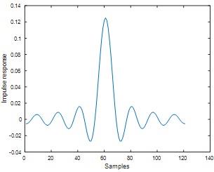
Fig 1
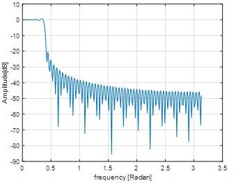
Fig 2
Question 2) Measure the filter frequency response at ωp = pi/8. Is it close to the expected value of -6dB? How much is the maximum ripple in the pass band.
Answer: 2)
MATLAB Code
lp=designfilt('lowpassfir','Filterorder',80,'CutoffFrequency',pi/8);
freqz(lp);
[fp wp]=freqz(lp);
figure
plot(wp/pi,db(fp));
xlabel('Normalized Frequency (\times\pi rad/sample)')
ylabel('Magnitude (dB)')
title('Frequency Response')
grid on
%% pass band rible
ps=0.02
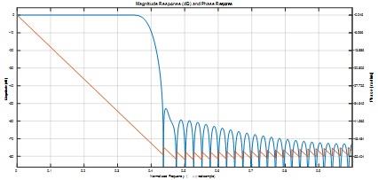
Fig 3
No , it's not close to -6 dB
Maximum pass band ripple is 0.01 dB
Question 3) This filtering technique does not define any cutoff. If we assume the stopband starts at -20dB, measure the ratio of the transient band to the pass band.
Answer: 3)
Ratio of transition band to passband=(stop band frequency of the filter- pass band frequency of the filter)/(pass band frequency of the filter)
From fig 2 we can seen that
Stop band frequency at -20 dB is 0.4
Transient band frequency is 0.4-0.35=0.05
Pass band frequency is 0.35
Ratio of transition band to passband = (0.4- 0.35)/0.35
=0.1429
GET GUARANTEED SATISFACTION OR MONEY BACK UNDER ME606 Z-TRANSFORMS AND FILTERS CONCEPTS ASSIGNMENT HELP SERVICES OF EXPERTSMINDS.COM - ORDER TODAY NEW COPY OF THIS ASSIGNMENT!
Question 4) Increase the filter impulse response length to M = 255 and run the program.
Answer: 4)
MATLAB Code
wp=pi/8; % lowpass filter bandwidth
M=255;
n=-(M-1)/2:(M-1)/2; % selection time window
h0=(wp/pi)*sinc((wp/pi)*n); % truncated impulse response
h=h0.*rectwin(M)'; % windowing
% h=h0.*hamming(M)';% windowing
% h=h0.*hanning(M)';% windowing
% h=h0.*bartlett(M)';% windowing
% h=h0.*blackman(M)';% windowing
figure;plot(h)
ylabel('Impulse response')
xlabel('Samples')
% spectrum
FFTsize=512;
pxx=20*log10(abs(fft(h,FFTsize)));
fxx=(0:(FFTsize/2)-1)*(pi/(FFTsize/2));
figure;plot(fxx,pxx(1:FFTsize/2));
ylabel('Amplitude[dB]');
xlabel('frequency [Radian]');grid on
lp=designfilt('lowpassfir','Filterorder',80,'CutoffFrequency',pi/8);
freqz(lp);
[fp wp]=freqz(lp);
figure
plot(wp/pi,db(fp));
xlabel('Normalized Frequency (\times\pi rad/sample)')
ylabel('Magnitude (dB)')
title('Frequency Response')
grid on
ps=0.01
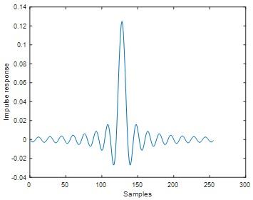
Fig 4
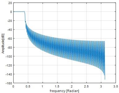
Fig 5
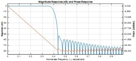
Fig 6
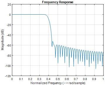
Fig 7
If we assume the stopband starts at -20dB, measure the ratio of the transient band to the passband.
a)
Ratio of transition band to passband=(stop band frequency of the filter- pass band frequency of the filter)/(pass band frequency of the filter)
From fig 5 we can seen that
Stop band frequency at -20 dB is 0.42
Transient band frequency is 0.42-0.4=0.02
Pass band frequency is 0.4
atio of transition band to passband = (0.42- 0.4)/0.4
=0.05
Measure the ripple in the passbad.
b) Pass band ripple is 0.015 dB
c) Discuss the effect of the filter length on the ripples and stopband attenuation.
c)
When the filter length M=121, ripple is 0.01 dB and the stop band attenuation is lesser than -20dB.if we increase the filter length from M=121 to 255, we got the ripple is 0.012 dB and the stop band attenuation is lesser than -20dB.When we increase the filter length we didn't get much variation of ripple and stop band attenuation. Ripple and stop band attenuation at filter length =121 and filter length=255 gives approximately same values.
24/7 AVAILABILITY OF TRUSTED ME606 Z-TRANSFORMS AND FILTERS CONCEPTS ASSIGNMENT WRITERS! ORDER ASSIGNMENTS FOR BETTER RESULTS!
Question 5) Use Hamming and Hanning window with the filter impulse response length, M=121, and discuss the effect of the window on the ripples and stopband attenuation.
Answer 5)
MATLAB code
M = 121;
wp=pi/8; % lowpass filter bandwidth
M=121;
n=-(M-1)/2:(M-1)/2; % selection time window
h0=(wp/pi)*sinc((wp/pi)*n); % truncated impulse response
% h=h0.*rectwin(M)'; % windowing
h=h0.*hamming(M)';% windowing
% h=h0.*hanning(M)';% windowing
% h=h0.*bartlett(M)';% windowing
% h=h0.*blackman(M)';% windowing
figure;plot(h)
ylabel('Impulse response')
xlabel('Samples')
% spectrum
FFTsize=512;
pxx=20*log10(abs(fft(h,FFTsize)));
fxx=(0:(FFTsize/2)-1)*(pi/(FFTsize/2));
figure;plot(fxx,pxx(1:FFTsize/2));
ylabel('Amplitude[dB]');
xlabel('frequency [Radian]');grid on
wp=pi/8; % lowpass filter bandwidth
M=121;
n=-(M-1)/2:(M-1)/2; % selection time window
h0=(wp/pi)*sinc((wp/pi)*n); % truncated impulse response
% h=h0.*rectwin(M)'; % windowing
% h=h0.*hamming(M)';% windowing
h=h0.*hanning(M)';% windowing
% h=h0.*bartlett(M)';% windowing
% h=h0.*blackman(M)';% windowing
figure;plot(h)
ylabel('Impulse response')
xlabel('Samples')
% spectrum
FFTsize=512;
pxx=20*log10(abs(fft(h,FFTsize)));
fxx=(0:(FFTsize/2)-1)*(pi/(FFTsize/2));
figure;plot(fxx,pxx(1:FFTsize/2));
ylabel('Amplitude[dB]');
xlabel('frequency [Radian]');grid on
Hamming window result
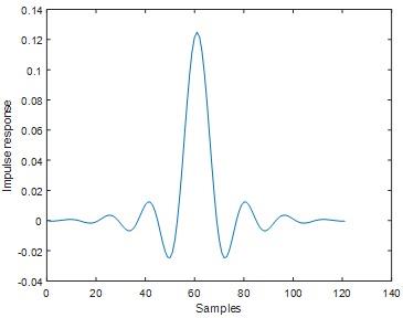
Fig 8
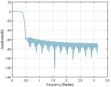
Fig 9
Hanning window result
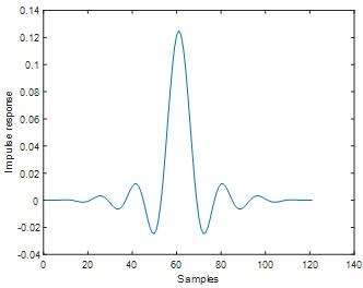
Fig 10
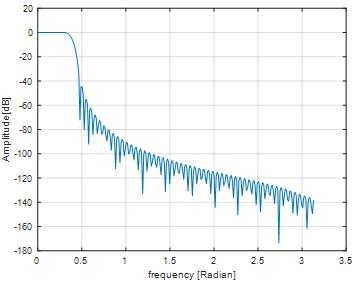
Fig 11
In both hamming and hanning window ripple is not exist.Stop band attenuation of hamming window is approximately equal to -60 dB and for hanning window Stop band attenuation is approximately equal to -44 dB. From these results we inferred, For the given filter length hamming window yields lesser stop band attenuation comparing to hanning window.
NEVER MISS YOUR CHANCE TO EXCEL IN ME606 Z-TRANSFORMS AND FILTERS CONCEPTS ASSIGNMENT! AVAIL AFFORDABLE AND RELIABLE ME606 DIGITAL SIGNAL PROCESSING ASSIGNMENTS HELP SERVICES OF EXPERTSMINDS.COM
Question 6) Change ωp=pi/4 and repeat 1) and discuss the effect.
Answer: 6)
MATLAB code
wp=pi/4; % lowpass filter bandwidth
M=121;
n=-(M-1)/2:(M-1)/2; % selection time window
h0=(wp/pi)*sinc((wp/pi)*n); % truncated impulse response
h=h0.*rectwin(M)'; % windowing
% h=h0.*hamming(M)';% windowing
% h=h0.*hanning(M)';% windowing
% h=h0.*bartlett(M)';% windowing
% h=h0.*blackman(M)';% windowing
figure;plot(h)
ylabel('Impulse response')
xlabel('Samples')
% spectrum
FFTsize=512;
pxx=20*log10(abs(fft(h,FFTsize)));
fxx=(0:(FFTsize/2)-1)*(pi/(FFTsize/2));
figure;plot(fxx,pxx(1:FFTsize/2));
ylabel('Amplitude[dB]');
xlabel('frequency [Radian]');grid on
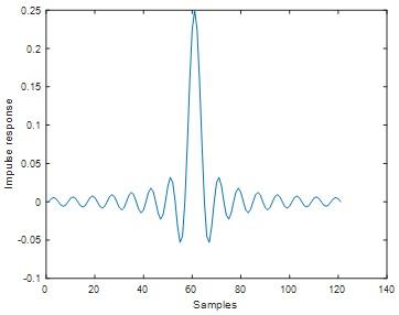
Fig 12
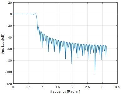
Fig 13
If we change the value of omega from pi/8 to pi/4 , Amplitude of the impulse response is increases,pass band and stop band frequency also increases.
1 -2 Designing a bandpass FIR filter using Windowed Fourier Series approach
Question 7) Run the above program and plot the impulse response and the amplitude spectrum of the filter.
Answer: 7)
MATLAB code
wp=pi/16; % lowpass filter bandwidth
M=121;
n=-(M-1)/2:(M-1)/2; % selection time window
h0=(wp/pi)*sinc((wp/pi)*n); % truncated impulse response
h1=h0.*rectwin(M)'; % windowing
w0=pi/4; % BPF center frequency
h=h1.*exp(j*w0*n); % Lowpass to bandpass conversion
figure; subplot(211);plot(real(h));ylabel('Real part of impulse response')
xlabel('samples')
subplot(212);plot(imag(h));ylabel('imag part of impulse response')
xlabel('samples') % spectrum
FFTsize=512;
pxx=20*log10(abs(fft(h,FFTsize)));
fxx=(0:(FFTsize/2)-1)*(pi/(FFTsize/2));
figure;plot(fxx,pxx(1:FFTsize/2));ylabel('Amplitude [dB]');xlabel('frequency [Radian]');grid on
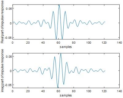
Fig 14
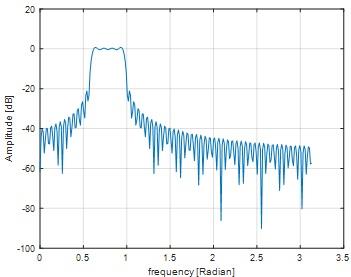
Fig 15
Question 8) What are the passband edges ωp1 ωp2. Measure the attenuation in frequency response at these frequencies and compare them with the expected value of -6dB.
Answer: 8)
Passband Edges
ωp1=0.53
ωp2=1
Attenuation using ωp1
A1=-20log10(ωp1)
A1=-20log10(0.53)
A1=5.5145
Attenuation using ωp2
A2=-20log10(1)
A2=-20log10(1)
A2=0
The attenuation of the passband edge ωp1 is nearly equal to 6 dB. The attenuation of the passband edge ωp2 is 0 dB which is not equal to 6 dB.
Question 9) Measure the maximum ripple in the passband.
Answer: 9)
Maximum ripple in the passband=0.01 dB
WE HELP STUDENTS TO IMPROVE THEIR GRADES! AVAIL TOP QUALITY ME606 Z-TRANSFORMS AND FILTERS CONCEPTS ASSIGNMENT HELP AND HOMEWORK WRITING SERVICES AT CHEAPER RATE!
Question 10) Increase ωp to pi/4 and discuss the result
Answer: 10)
MATLAB code
wp=pi/4; % lowpass filter bandwidth
M=121;
n=-(M-1)/2:(M-1)/2; % selection time window
h0=(wp/pi)*sinc((wp/pi)*n); % truncated impulse response
h1=h0.*rectwin(M)'; % windowing
w0=pi/4; % BPF center frequency
h=h1.*exp(j*w0*n); % Lowpass to bandpass conversion
figure; subplot(211);plot(real(h));ylabel('Real part of impulse response')
xlabel('samples')
subplot(212);plot(imag(h));ylabel('imag part of impulse response')
xlabel('samples') % spectrum
FFTsize=512;
pxx=20*log10(abs(fft(h,FFTsize)));
fxx=(0:(FFTsize/2)-1)*(pi/(FFTsize/2));
figure;plot(fxx,pxx(1:FFTsize/2));ylabel('Amplitude [dB]');xlabel('frequency [Radian]');grid on
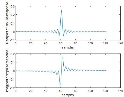
Fig 16
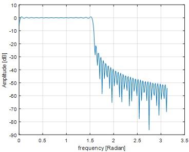
Fig 17
When the frequency of ωp is increased into pi/4, the passband edges lying between 0.1 to 1.6.The transition bandwith also increased.The ripple remains same like before.
ENDLESS SUPPORT IN ME606 Z-TRANSFORMS AND FILTERS CONCEPTS ASSIGNMENTS WRITING SERVICES - YOU GET REVISED OR MODIFIED WORK TILL YOU ARE SATISFIED WITH OUR ME606 DIGITAL SIGNAL PROCESSING ASSIGNMENT HELP SERVICES!
1 -3 Designing a band-stop FIR filter using Frequency sampling approach
Question 11) Report your MATLAB code. Select the filter impulse response length M=121;
Answer: 11)
MATLAB code
wp=pi/8; % filter bandwidth
M=121;
n=-(M-1)/2:(M-1)/2; % selection time window
h0=(wp/pi)*sinc((wp/pi)*n); % truncated impulse response
h1=h0.*rectwin(M)'; % windowing
w0=pi/4; % BPF center frequency
h=h1-(h1.*exp(j*w0*n)); %band stop filter
figure; subplot(211);plot(real(h));ylabel('Real part of impulse response')
xlabel('samples')
subplot(212);plot(imag(h));ylabel('imag part of impulse response')
xlabel('samples')
FFTsize=512;
pxx=20*log10(abs(fft(h,FFTsize)));
fxx=(0:(FFTsize/2)-1)*(pi/(FFTsize/2));
figure;plot(fxx,pxx(1:FFTsize/2));ylabel('Amplitude [dB]');xlabel('frequency [Radian]');grid on
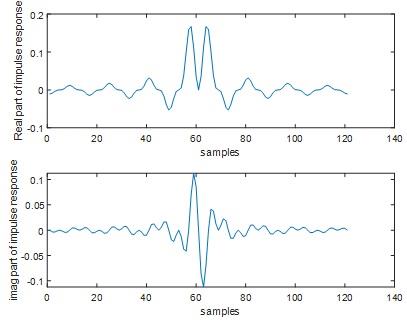
Fig 18
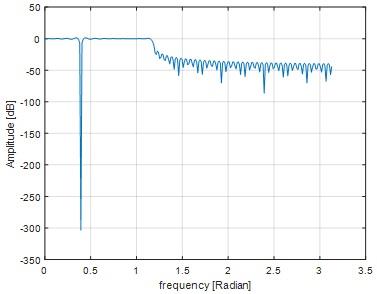
Fig 19
Question 12) Plot the frequency response, |H(ejω)|, of your filter on the top of the spectrum mask in a single plot.
Answer: 12)
MATLAB code
bs = fdesign.bandstop('Fp1,Fst1,Fst2,Fp2,Ap1,Ast,Ap2', ...
pi/4,pi/3.8,pi/3.5,1,1,60,1);
bs1 = design(bs);
freqz(bs1);
[fp wp]=freqz(bs1);
figure
plot(wp/pi,db(fp));
xlabel('Normalized Frequency (\times\pi rad/sample)')
ylabel('|H(e^(j?))|')
title('Frequency Response')
grid on
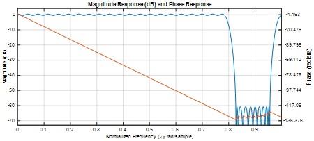
Fig 20
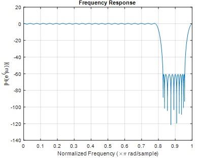
Fig 21
Question 13) Plot 20*log10(|H(ejω)|) of your filter on the top of the spectrum mask in dB in a single plot.
Answer: 13)
MATLAB code
bs = fdesign.bandstop('Fp1,Fst1,Fst2,Fp2,Ap1,Ast,Ap2', ...
pi/4,pi/3.8,pi/3.5,1,1,60,1);
bs1 = design(bs);
freqz(bs1);
[fp wp]=freqz(bs1);
figure
plot(wp/pi,20*log10(db(fp)));
xlabel('Normalized Frequency (\times\pi rad/sample)')
ylabel('|H(e^jw)| in dB')
title('Frequency Response')
grid on
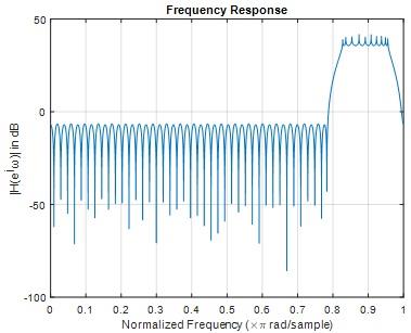
Fig 22
Question 14) Measure the amplitude at ω = [Π/4, 3Π/4, Π/2] on your second plot.
Answer: 14)
MATLAB code
wp=pi/8; % lowpass filter bandwidth
M=121;
n=-(M-1)/2:(M-1)/2; % selection time window
h0=(wp/pi)*sinc((wp/pi)*n); % truncated impulse response
h1=h0.*rectwin(M)'; % windowing
w0=(pi)/4; % BPF center frequency
h=h1-(h1.*exp(j*w0*n)); %band stop filter
FFTsize=512;
pxx=20*log10(abs(fft(h,FFTsize)));
fxx=(0:(FFTsize/2)-1)*(pi/(FFTsize/2));
figure;plot(fxx,pxx(1:FFTsize/2));ylabel('Amplitude [dB]');xlabel('frequency [Radian]');grid on
wp=pi/8; % lowpass filter bandwidth
M=121;
n=-(M-1)/2:(M-1)/2; % selection time window
h0=(wp/pi)*sinc((wp/pi)*n); % truncated impulse response
h1=h0.*rectwin(M)'; % windowing
w0=(3*pi)/4; % BPF center frequency
h=h1-(h1.*exp(j*w0*n)); %band stop filter
FFTsize=512;
pxx=20*log10(abs(fft(h,FFTsize)));
fxx=(0:(FFTsize/2)-1)*(pi/(FFTsize/2));
figure;plot(fxx,pxx(1:FFTsize/2));ylabel('Amplitude [dB]');xlabel('frequency [Radian]');grid on
wp=pi/8; % lowpass filter bandwidth
M=121;
n=-(M-1)/2:(M-1)/2; % selection time window
h0=(wp/pi)*sinc((wp/pi)*n); % truncated impulse response
h1=h0.*rectwin(M)'; % windowing
w0=(pi)/2; % BPF center frequency
h=h1-(h1.*exp(j*w0*n)); %band stop filter
FFTsize=512;
pxx=20*log10(abs(fft(h,FFTsize)));
fxx=(0:(FFTsize/2)-1)*(pi/(FFTsize/2));
figure;plot(fxx,pxx(1:FFTsize/2));ylabel('Amplitude [dB]');xlabel('frequency [Radian]');grid on
Omega=pi/4
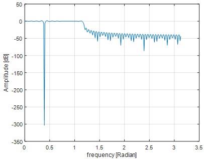
Fig 23
Omega=3*pi/4
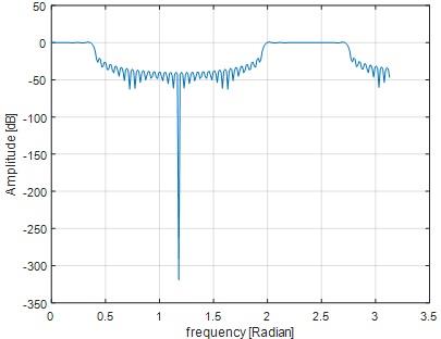
Fig 24
Omega=pi/2
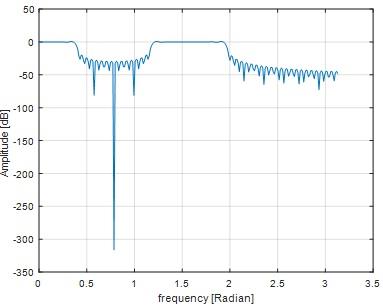
Fig 25
Question 15) Find the deepest point in your frequency response in dB. How you can increase the depth of the stopband?
Answer: 15)
Deepest point in frequency response is 0.88.By increasing the value of cutoff frequency we can increase the depth of stop band.
1-4 Designing a low pass FIR filter using Frequency sampling approach
Question 16) Run the above program and plot the impulse response and the amplitude spectrum of the filter. Try to understand what the program does.
Answer: 16)
MATLAB code
wp=pi/8;
M=121;
FFTsize=512; % passband frequency samples
Np=fix((wp/(2*pi))*FFTsize); % number of pass band samples
Ns=FFTsize/2-Np; % number of stop band samples
H1=[ones(1,Np) zeros(1,Ns+1)];
H=[H1 H1(end:-1:2)]; % sampled frequency spectrum;
fxx=(0:(FFTsize/2)-1)*(pi/(FFTsize/2));
figure;plot(fxx,H(1:FFTsize/2));
ylabel('Amplitude'); xlabel('frequency [Radian]');grid on
% finding impulse response by truncating
h1=real(ifft(H));
h0=[ h1(end-(M-1)/2+1:end) h1(1:1+(M-1)/2)];
figure;plot(h0)
ylabel('Impulse response')
xlabel('Samples')
% spectrum
pxx=20*log10(abs(fft(h0,FFTsize)));
fh=figure;plot(fxx,pxx(1:FFTsize/2));hold on;
% effect of windowing
h=h0.*hanning(M)';% windowing
% spectrum
pxx=20*log10(abs(fft(h,FFTsize)));
figure(fh);plot(fxx,pxx(1:FFTsize/2));grid on; legend('rectwin','hanning')
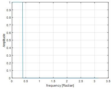
Fig 26
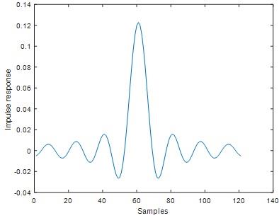
Fig 27
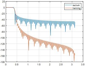
Fig 28
Question 17) Use the above program as your base, design a band pass filter that passes the frequencies between pi/8<w<pi/4. Only modify the lines 5-7 and do not touch the rest of the program.
Answer: 17)
MATLAB code
wp=pi/8;
wp1=pi/4;
M=121;
FFTsize=512; % passband frequency samples
Np=fix((wp/(2*pi))*FFTsize); % number of pass band samples
Ns=fix((wp1/(2*pi))*FFTsize); % number of stop band samples
H1=[zeros(1,Np) ones(1,Ns+1) zeros(1,Np) ];
H=[H1 H1(end:-1:2)]; % sampled frequency spectrum;
fxx=(0:(FFTsize/2)-1)*(pi/(FFTsize/2));
figure;plot(fxx,H(1:FFTsize/2));
ylabel('Amplitude'); xlabel('frequency [Radian]');grid on
% finding impulse response by truncating
h1=real(ifft(H));
h0=[ h1(end-(M-1)/2+1:end) h1(1:1+(M-1)/2)];
figure;plot(h0)
ylabel('Impulse response')
xlabel('Samples')
% spectrum
pxx=20*log10(abs(fft(h0,FFTsize)));
fh=figure;plot(fxx,pxx(1:FFTsize/2));hold on;
% effect of windowing
h=h0.*hanning(M)';% windowing
% spectrum
pxx=20*log10(abs(fft(h,FFTsize)));
figure(fh);plot(fxx,pxx(1:FFTsize/2));grid on; legend('rectwin','hanning')
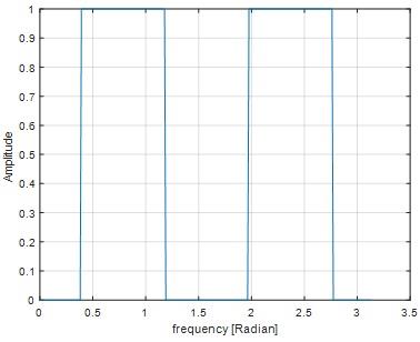
Fig 29
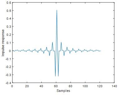
Fig 30
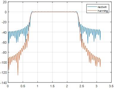
Fig 31
EXPERTSMINDS.COM GIVES ACCOUNTABILITY OF YOUR TIME AND MONEY - AVAIL TOP RESULTS ORIGINATED ME606 DIGITAL SIGNAL PROCESSING ASSIGNMENT HELP SERVICES AT BEST RATES!
Section 2. Analyzing a system in Z and time domain
Question 18) Assume the system is causal. Draw its region of convergence (ROC) in the z-plane
Answer: 18)
MATLAB code
nm=[1 -0.2];
dm=[1 -0.8 0.15]
[a b c]=tf2zp(nm,dm);
zplane(nm,dm);
H(z)=(1-0.2z^(-1))/((1-0.5z^(-1) )(1-0.3z^(-1)))
H(z)=(1-0.2z^(-1))/((1-0.3z^(-1)-0.5z^(-1) )+0.15z^(-2)))
H(z)=(1-0.2z^(-1))/((1-0.8z^(-1) )+0.15z^(-2)))
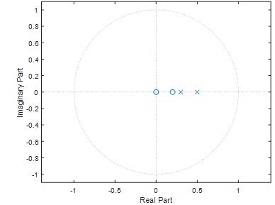
Fig 32
Question 19) Is the system stable or unstable? Why?
Answer: 19)
The given system is stable.From the Fig 32 we can see that all the poles are inside the unit circle. Therefore the system is said to be stable.
Question 20) Determine the system difference equation in the form of
∑k=0N akY[n-k] = ∑k=0M bkx[n-k]
Answer: 20)
H(z)=(1-0.2z^(-1))/((1-0.8z^(-1) )+0.15z^(-2)))
H(z)=Y(z)/X(z)
Y(z)/X(z)=(1-0.2z^(-1))/((1-0.8z^(-1) )+0.15z^(-2)))
(1-0.8z^(-1)+0.15z^(-2) )Y(z)=(1-0.2z^(-1)) X(z)
Y(z)-0.8z^(-1) Y(z)+0.15z^(-2) Y(z)=X(z)-0.2z^(-1) X(z)
u(n)-0.8y(n-1)+0.15y(n-2)=u(n)-0.2x(n-1)
0.8y(n-1)-0.15y(n-2)=0.2x(n-1)
-5.3[y(n-1)+y(n-2)]=-1.3x(n-1)
∑_(k=0)^2?y(n-k)=? ∑_(k=0)^1x(n-k)
Question 21) Give the values for ai and bj , N and M
Answer: 21)
ai=-5.3
bi=-1.3
N=2
M=1
Question 22) Sketch the magnitude of the frequency response of the system between 0 and Π
Answer 22)
MATLAB code
b=[1 -0.2];
a1=[1 -0.5];
a2=[1 -0.3];
ak=conv(a1,a2);
freqz(b,ak,1000)
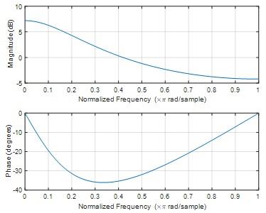
Fig 33
Question 23) Suppose the above transfer function is a filter, what type of filter is it?
Question Answer 23)
Low pass filter
Question 24) Sketch a block diagram for implementing this system
Answer 24)
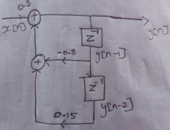
Question Answer 25) Find the system causal impulse response
Answer 25)
MATLAB code
nm=[1 -0.2];
dm=[1 -0.8 0.15]
[p q r]=residue(nm,dm)
gg=tf(p',q');
figure
impulse(gg)
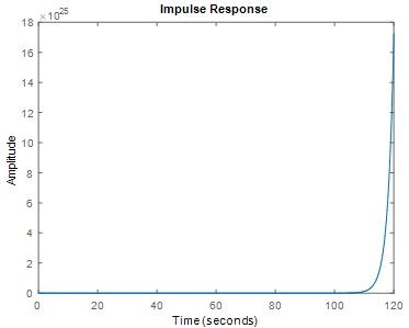
Fig 34
Question 26) Assume the initial condition is zero, enter a unit impulse to the system and find the impulse response of the system h[n] for the first 10 samples and compare it with the step11
Answer 26)
MATLAB code
nm=[1 -0.2];
dm=[1 -0.8 0.15]
figure
impz(nm,dm)
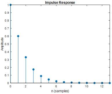
Fig 35
Section 3. Filtering
Question 27) Plot and include the plot in your report. Simply, mention the application of the "pwelch" program, and what are its input parameters.
Answer 27)
MATLAB code
x=randn(1,5000); % signal to be filtered
NFFT=512; % FFTT size (N)
overlap_samples=0; % number of overlap samples in time frames
y=conv(x,h); % filtering operation using convolution
[Pxx,W] = pwelch(y,hamming(NFFT),overlap_samples,NFFT);
figure;plot(W,Pxx);
xlabel('W [radian] from 0-pi');ylabel(' power spectral density')
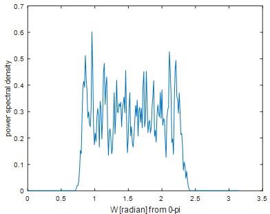
Fig 36
Application of Pwelch
signal simulation and measurements
noise simulation and measurements
In the field of dividing signal into segments
Input parameters of Pwelch
1. Input signal
2. Window
3. Noverlap samples
4. Number of DFT points
Question 28) Measure the filter delay and find a ratio of the filter delay to the filter impulse response length
Answer: 28)
MATLAB code
x=[-zeros(1,500) ones(1,1000) zeros(1,500)]; % signal to be filtered
y=conv(x,h); % filtering operation using convolution
figure;plot(x,'.-')
hold on;
plot(y,'.-'); grid; xlabel('sample')
legend('filter input signal','filter output')
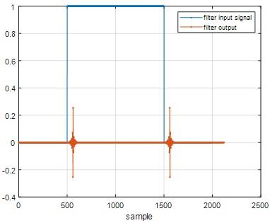
Fig 37
From fig 37 we can obtain,
Filter delay= 0.23 secs
Filter impulse response length=1000
Ratio= Filter delay/ Filter impulse response length =2.3*10-4
SAVE DISTINCTION MARKS IN EACH ME606 Z-TRANSFORMS AND FILTERS CONCEPTS ASSIGNMENT WHICH IS WRITTEN BY OUR PROFESSIONAL WRITER!
Get our Melbourne Institute of Technology Assignment Help for the below mentioned courses like:-
- ME700 Industry Experience Assignment Help
- MN506 System Management Assignment Help
- ME603 Project Assignment Help
- MN503 Overview of Internetworking Assignment Help
- MN605 Enterprise Network Design Assignment Help
- ME503 Telecommunication System Engineering Assignment Help
- ME501 Professional Engineering Practice Assignment Help
- ME602 Mobile and Satellite Communication Systems Assignment Help
- ME693 Software-Defined Radio Communication Assignment Help
- ME601 Telecommunication Modeling and simulation Assignment Help